Computational graph

A computational graph is essentially a sequence of operations that are applied on values. Mathematical equations can be broken down into a set of smaller steps, and we can treat those steps as nodes on a computational graph. Take for instance the following equation.

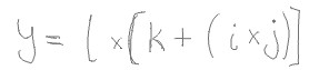
We can express this equation as a computational graph as follows.

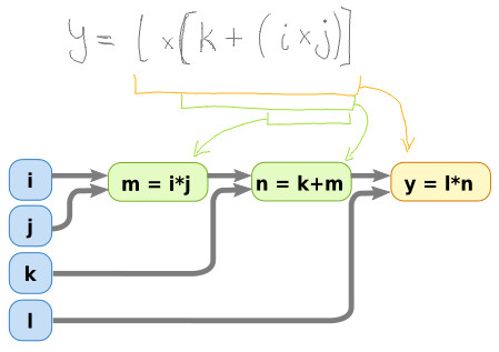
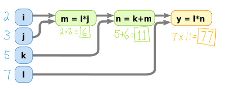
If we plug in some values for the input variables, i,j,k and l then we can calculate what the output should be.

Naive partial derivatives along a computational graph

A derivative simply calculates the rate of change at some particular point. A partial derivative refers to the rate of change that a specific input variable is responsible for. To put it more concretely, imagine we wish to calculate how much the output will change, if we modify one of the input variables by some very tiny amount. This ratio, of the difference in output, over the difference in one of the variables, is the partial derivative.

We can perform a naive calculation of the partial derivative as follows:

1. Plug in the input values
2. Plug in the same input values, except for the variable we want to calculate the partial derivative for. Increment its value by some very tiny amount.
3. Compare the difference in the output value, and the differences in input value for the desired variable.

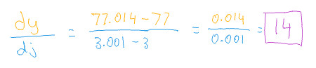
For example, if we change the variable j by a tiny amount of 0.001, we get the following output value:

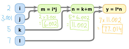
Which allows us to calculate the rate of change.

Partial derivatives using calculus

We can make use of the chain rule from calculus to calculate the partial derivative of the output with respect to any of the input variables. The way it can be broken down into several components is as follows:

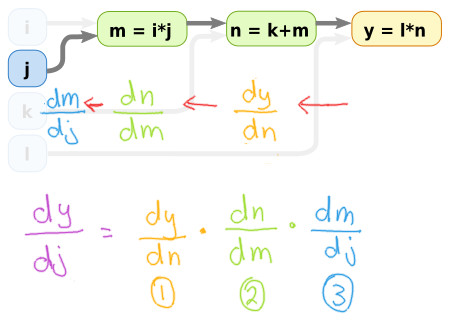
This now makes the problem of calculating the derivatives a lot easier, since we only need to consider small sub-problems at a time.

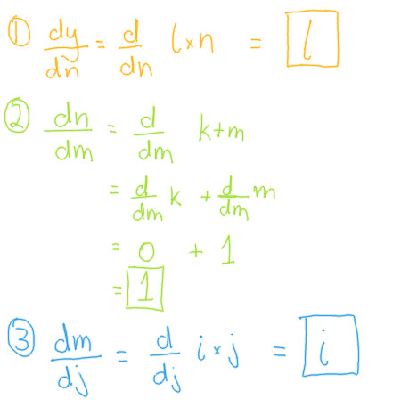
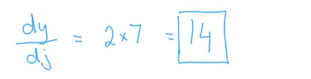
Now that those sub-problems have been solved, we can substitute then back in to our chain rule to get the partial derivative of our chosen variable.

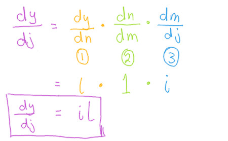
Voila! we now have a formula for calculating the partial derivative of the output, with respect to the chosen variable j, that will work no matter what values we have for any of the input variables.

We can test this on the input values we used previosuly and compare it against the result we got for the naive partial derivative.

We get the exact same result.

Checking on PyTorch

One of the beautiful things about PyTorch is that it makes inspecting the partial derivatives along a computational graph so incredibly easy.

from torch import Tensor
from torch.autograd import Variable

def element(val):
    return Variable(Tensor([val]), requires_grad=True)

# Input nodes
i = element(2)
j = element(3)
k = element(5)
l = element(7)

# Middle and output layers
m = i*j
n = m+k
y = n*l

# Calculate the partial derivative
y.backward()
dj = j.grad
print(dj)

Which gives the following output:

Variable containing:
 14
[torch.FloatTensor of size 1]

We can see that it matches all our previous calculations we did by hand :)