ERFNet Segmentation Model
A model for semantic segmentation that recently came out is the Efficient Residual Factorized Network (ERFNet) (Romera et al 2017a, Romera et al 2017b) which combines the ideas from several high performing deep neural network architectures in order to create an efficient, and powerful architecture for the semantic segmentation task.
The purpose of this project was to implement this architecture from scratch in Tensroflow, based on the description in the academic paper.
The model was trained on the CamVid dataset and achieved an IOU score of 0.485 on a portion of the dataset it did not see during training.
The Architecture
The ERFNet architecture makes use of three different modules that it stacks together.
- A factorized residual network module with dilations.
- A downsampling module inspired by an inception module.
- An upsampling module.
Each of these will be explained in the following subsections.
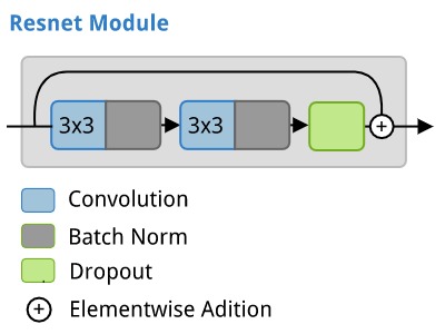
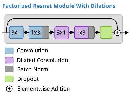
Factorized Resnet Modules with Dilation
Residual networks (He et al. 2015) have been incredibly successful for computer vision tasks. They allow for very deep models to be created without as much risk of vanishing/exploding gradients. ERFNet makes use of Resnet modules but modifies them with the addition of two other deep learning techniques. It makes use of asymmetric factorized convolutions (Szegedy et al 2015) to make it more computationally efficient. It also makes use of dilated convolutions (Yu and Koltun 2015) to give the layers in the network a lot of context.
A standard residual network module looks like this:
In an ERFNet, the residual modules with factorized, and dilated convolutions looks like this:
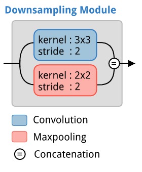
Downsampling Module
The inception network (Szegedy et al. 2014) makes use of multiple branches, each which undergo a different operation. The resulting outputs then get concatenated together to form the output of the module. This idea is used by ERFNet for the downsampling module. It splits the input into two branches. On one branch, a convolutional operation with a stride of 2 is applied, and along the other branch, a max-pooling operation is applied.
Upsampling Module
The upsampling module is just a fractionally strided convolution (aka inverse convolution, or deconvolution).
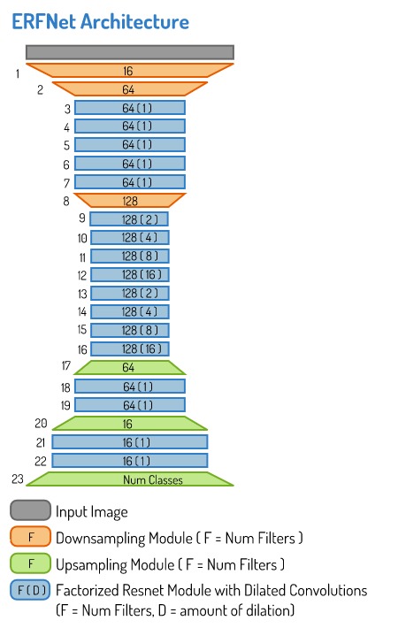
Complete Architecture
The ERFNet combines the above modules in the following arrangement.
Implementation
The model was implemented in tensorflow 1.3.
Data
The Cambridge-driving Labeled Video Database (CamVid) is a dataset that contains 701 Images captured from the perspective of a car driving on the roads of Cambridge, UK. The images are labeled with 32 semantic classes that include things like the road, footpath, cars, pedestrians, traffic signs, etc.
Input Data
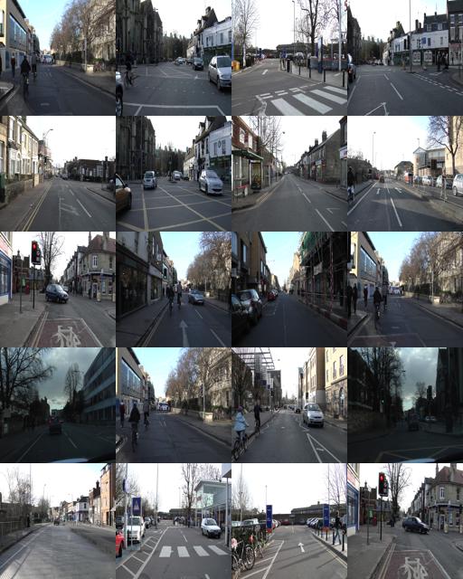
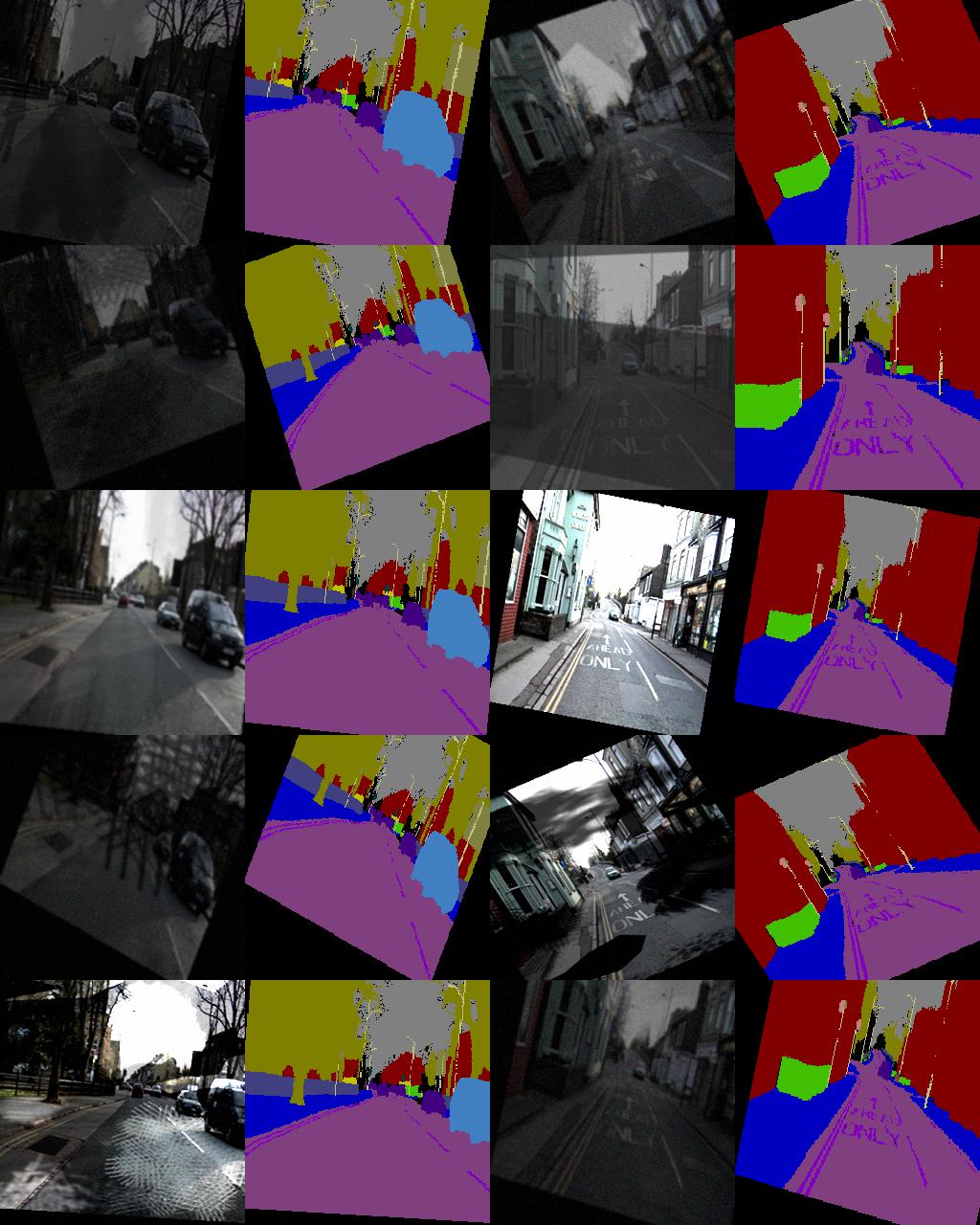
The input images are RGB png images with dimensions of 960x720. Below is a sample of 20 images from the dataset.
Labels
The labels are also encoded as RGB PNG images, with each of the 32 semantic classes represented as a different RGB value.
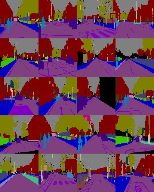
The mapping of the different semantic classes is as follows:
| Animal (64, 128, 64) | |
| Archway (192, 0, 128) | |
| Bicyclist (0, 128, 192) | |
| Bridge (0, 128, 64) | |
| Building (128, 0, 0) | |
| Car (64, 0, 128) | |
| CartLuggagePram (64, 0, 192) | |
| Child (192, 128, 64) | |
| Column_Pole (192, 192, 128) | |
| Fence (64, 64, 128) | |
| LaneMkgsDriv (128, 0, 192) | |
| LaneMkgsNonDriv (192, 0, 64) | |
| Misc_Text (128, 128, 64) | |
| MotorcycleScooter (192, 0, 192) | |
| OtherMoving (128, 64, 64) | |
| ParkingBlock (64, 192, 128) | |
| Pedestrian (64, 64, 0) | |
| Road (128, 64, 128) | |
| RoadShoulder (128, 128, 192) | |
| Sidewalk (0, 0, 192) | |
| SignSymbol (192, 128, 128) | |
| Sky (128, 128, 128) | |
| SUVPickupTruck (64, 128, 192) | |
| TrafficCone (0, 0, 64) | |
| TrafficLight (0, 64, 64) | |
| Train (192, 64, 128) | |
| Tree (128, 128, 0) | |
| Truck_Bus (192, 128, 192) | |
| Tunnel (64, 0, 64) | |
| VegetationMisc (192, 192, 0) | |
| Void (0, 0, 0) | |
| Wall (64, 192, 0) |
Distribution of classes
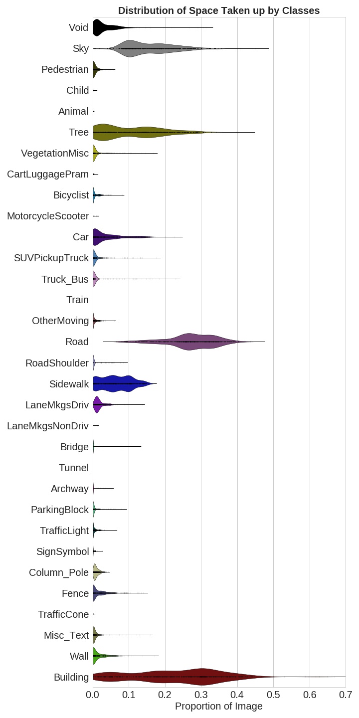
The distribution of how much of the image each class takes (as a proportion of the number of pixels in the image) can be viewed in the following plot. We can see that buildings, roads, sky, and trees disproportionately dominate the scenes, and other classes occur with much less frequency.
Data Preparation
Resizing Input images
The input images were resized and reshaped to 256*256 in dimensions, and stored in numpy arrays of shape [n_samples,256,256,3].
Label images
The label images were also resized to 256*256 in dimensions. But in order to be useful for training a deep learning model, they had to be converted from RGB images to single-channel images, with the integer value for each pixel representing the class ID. These were also stored in numpy arrays, but of shape [n_samples, 256,256].
Train/validation split
Out of the 701 samples in the data, 128 were put aside at random to for the validation set. This left 573 images remaining for the training set.
The resulting data had the following shapes:
| Dataset | shape |
|---|---|
X_valid |
[128, 256, 256, 3] |
Y_valid |
[128, 256, 256] |
X_train |
[573, 256, 256, 3] |
Y_train |
[573, 256, 256] |
Data Augmentation
Since the training set was quite small, data augmentation was needed for training in order to allow the model to generalize better.
The following data augmentation steps were taken:
- shadow augmentation: with random blotches and shapes of different intensities being overlayed over the image.
- random rotation: between -30 to 30 degrees
- random crops: between 0.66 to 1.0 of the image
- random brightness: between 0.5 and 4, with a standard deviation of 0.5
- random contrast: between 0.3 and 5, with a standard deviation of 0.5
- random blur: randomly apply small amount of blur
- random noise: randomly shift the pixel intensities with a standard deviation of 10.
Below is an example of two training images (and their accompanying labels) with data augmentation applied to them five times.
Class weighting
Since the distribution of classes on the images is quite imbalanced, class weighting was used to allow the model to learn about objects that it rarely sees, or which take up smaller regions of the total image. The method used was is from Paszke et al 2016
weight_class = 1/ln(c + class_probability)
Where:
cis some constant value that is manually set. As per Romera et al 2017a, a value of1.10was used.
The table below shows the weight applied to the different classes when this formula is used. Greater weight is given to smaller or rarer objects, eg child (10.46), than objects that occur more often and consume large portions of the image, eg sky (4.37).
| Class | Weight |
|---|---|
| Void | 8.19641542163 |
| Sky | 4.3720296426 |
| Pedestrian | 9.88371158915 |
| Child | 10.4631076496 |
| Animal | 10.4870856376 |
| Tree | 5.43594061016 |
| VegetationMisc | 9.77766487673 |
| CartLuggagePram | 10.4613353846 |
| Bicyclist | 9.99897358787 |
| MotorcycleScooter | 10.4839211216 |
| Car | 7.95097080927 |
| SUVPickupTruck | 9.7926997517 |
| Truck_Bus | 10.0194993159 |
| Train | 10.4920586873 |
| OtherMoving | 10.1258833847 |
| Road | 3.15728309302 |
| RoadShoulder | 10.2342992955 |
| Sidewalk | 6.58893008318 |
| LaneMkgsDriv | 9.08285926082 |
| LaneMkgsNonDriv | 10.4757462996 |
| Bridge | 10.4371404226 |
| Tunnel | 10.4920560223 |
| Archway | 10.4356039685 |
| ParkingBlock | 10.1577327692 |
| TrafficLight | 10.1479245421 |
| SignSymbol | 10.3749043447 |
| Column_Pole | 9.60606490919 |
| Fence | 9.26646394904 |
| TrafficCone | 10.4882678542 |
| Misc_Text | 9.94147719336 |
| Wall | 9.32269173889 |
| Building | 3.47796865386 |
Training
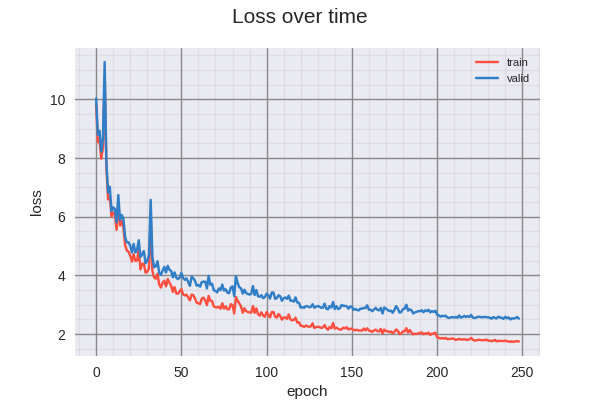
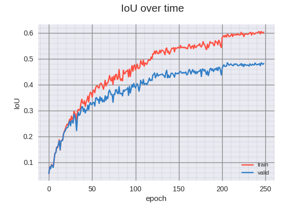
The model was trained for 249 epochs, a snapshot was taken of the model after completing each epoch. An additional snapshot was taken if the IOU score evaluated on the validation dataset was higher than any previous epoch. This allowed the best version of the model to be preserved in the case that further training caused the model to get worse.
The training schedule was as folows:
| learning rate | num epochs |
|---|---|
| 8e-4 | 80 |
| 5e-4 | 80 |
| 2e-4 | 40 |
| 1e-4 | 40 |
| 5e-5 | 40 |
The final one was terminated early (after just 9 epochs) since it was not making the model any better on the validation dataset.
The training curves can be seen below.
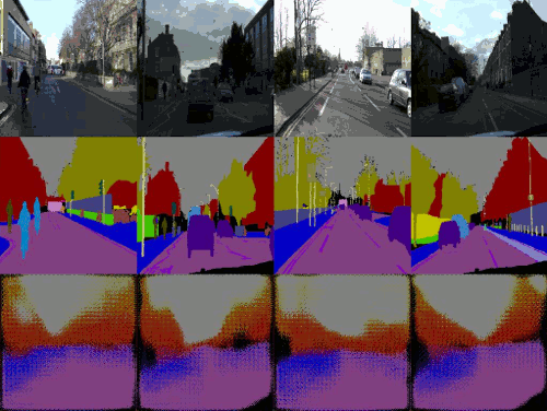
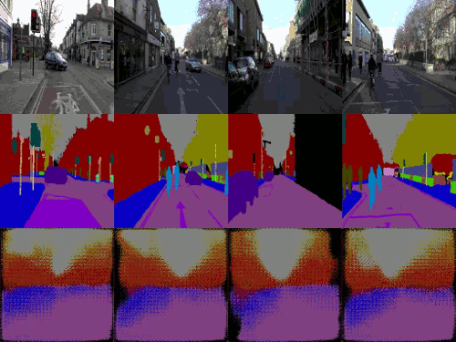
The following animated GIF illustrates the evolution of the predictions made (on training dataset) as the model trains. The top row contains the input image, the middle row contains the ground truth, and the bottom row contains the predictions made by the mode. Each timeframe in the animation represents 3 elapsed epochs.
The following animated GIF is of the predictions on the validation dataset.
Results and Discussion
The best version of the model was achieved in epoch 206, attaining the following scores:
| Mertic | Value |
|---|---|
| IOU (valid) | 0.48511058 |
| IOU (train) | 0.59533381 |
| Loss (valid) | 2.5678083598613739 |
| Loss (train) | 1.8275435666243236 |
There is clearly overfitting occurring in this model. Perhaps with slightly more aggressive regularization, this could be reduced. Visually, however, the results are quite impressive.
Future work
One of the appealing things about this architecture is that it was designed to be capable of running in real time on a GPU. According to Romera et al 2017a and Romera et al 2017b it should be capable of running at 83 FPS in a single Titan X, and at more than 7 FPS in a Jetson TX1 embedded GPU. I would like to come back to this architecture to see if it can be optimized to run in real time on a laptop with no GPU, or an Android device.
Links
- Source Code hosted on Github
Credits
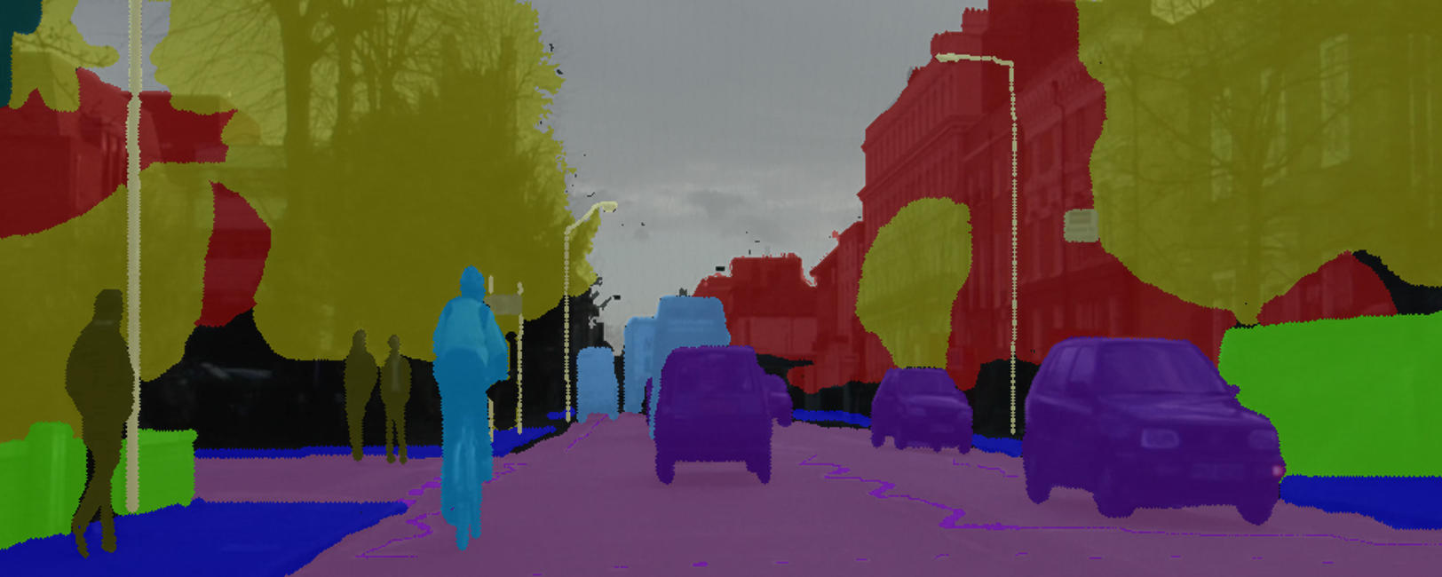
- Image for the banner is an overlay of a training image and label image from the Camvid Dataset