Creating Birdseye View of Point Cloud Data
Relevant axes for Birds Eye Views
In order to create a birdseye view image, the relevant axes from the point cloud data will be the x and y axes.
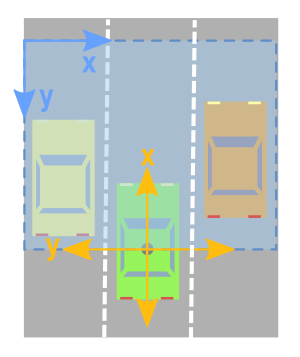
However, as we can see from the image above, we have to be careful and take the following things into consideration:
- the x, and y axes mean the opposite thing.
- The x, and y axes point in the opposite direction.
- You have to shift the values across so that (0,0) is the smallest possible value in the image.
Limiting Rectangle to Look at
It is often useful to just concentrate on a specific region of the point cloud. As such, we will want to create a filter that only keeps the points that are within the region we are interested in.
Since we are looking at the data from the top and we are interested in converting it to an image, I will be using directions that are a bit more consistent with image axes. Below, I specify the range of values I want to concentrate on relative to the origin. Anything to the left of the origin will be considered negative, and anything to the right as positive. The x axis of the point cloud will be interpreted as the forward direction (which will be the upwards direction of our birds eye image).
The code below sets the rectangle of interest to span 10m on either side of the origin, and 20m in front of it.
side_range=(-10, 10)     # left-most to right-most
fwd_range=(0, 20)       # back-most to forward-most
Next, we create a filter, to only keep the points that actually lie within the rectangle we specified.
# EXTRACT THE POINTS FOR EACH AXIS
x_points = points[:, 0]
y_points = points[:, 1]
z_points = points[:, 2]

# FILTER - To return only indices of points within desired cube
# Three filters for: Front-to-back, side-to-side, and height ranges
# Note left side is positive y axis in LIDAR coordinates
f_filt = np.logical_and((x_points > fwd_range[0]), (x_points < fwd_range[1]))
s_filt = np.logical_and((y_points > -side_range[1]), (y_points < -side_range[0]))
filter = np.logical_and(f_filt, s_filt)
indices = np.argwhere(filter).flatten()

# KEEPERS
x_points = x_points[indices]
y_points = y_points[indices]
z_points = z_points[indices]
Mapping Point Positions to Pixel Positions
At the moment, we have a bunch of points that take on real number values. In order to map those to map those values to integer position values. We could just naively typecast all the x and y values to integers, but we might end up losing a lot of resolution. For instance, if the unit of measurement for those points is in metres, then each pixel would represent an rectangle that is 1x1 metre in the point cloud, and we would lose any detail smaller than this. This might be fine if you have a point cloud of something like a mountainscape. But if you want to be able to capture finer details and recognize things like humans, and cars, or even smaller things, then this method is no good.
However, the above method can be modified slightly so that we get the level of resolution we desire. We can just scale the data first, before typecasting to integers. If for instance the unit of measurement was in metres, and we want a resolution of 5cm, we can do something like the following:
res = 0.05
# CONVERT TO PIXEL POSITION VALUES - Based on resolution
x_img = (-y_points / res).astype(np.int32)  # x axis is -y in LIDAR
y_img = (-x_points / res).astype(np.int32)  # y axis is -x in LIDAR
You would have noticed that the x and y axes were swapped, and direction reversed so that we can now start dealing with image coordinates.
Shifting to New Origin
The x and y data is still not quite ready to be mapped to an image. We may still have negative x and y values. So we need to shift the data to make (0,0) the smallest value.
# SHIFT PIXELS TO HAVE MINIMUM BE (0,0)
# floor and ceil used to prevent anything being rounded to below 0 after shift
x_img -= int(np.floor(side_range[0] / res))
y_img += int(np.ceil(fwd_range[1] / res))
And we can probe the data to prove to ourselves that the values are all now positive, eg:
>>> x_img.min()
7
>>> x_img.max()
199
>>> y_img.min()
1
>>> y_img.max()
199
Pixel Values
So we have used the point data to specify x and y positions in the image. What
we need to do now is specify what value we want to fill those pixel positions
with. One possibility is to populate it with the height data. Two things to
keep in mind though are:
- Pixel values should be integers.
- Pixel values should be values between the range 0-255.
We could take the min and max height value from the data, and re-scale that range to fit within the range of 0-255. Another approach, one which will be used here is to set a range of height values we want to concentrate on, and anything above or below that range gets clipped to the min and max values. This is useful since it allows us to get the maximum amount of detail from a region of interest.
In the following code, we set the range to be 2 metres below the origin, and half a meter above it.
height_range = (-2, 0.5)  # bottom-most to upper-most

# CLIP HEIGHT VALUES - to between min and max heights
pixel_values = np.clip(a = z_points,
                           a_min=height_range[0],
                           a_max=height_range[1])
Next we re-scale those values to be between 0-255, and typecast to integers.
def scale_to_255(a, min, max, dtype=np.uint8):
    """ Scales an array of values from specified min, max range to 0-255
        Optionally specify the data type of the output (default is uint8)
    """
    return (((a - min) / float(max - min)) * 255).astype(dtype)

# RESCALE THE HEIGHT VALUES - to be between the range 0-255
pixel_values  = scale_to_255(pixel_values, min=height_range[0], max=height_range[1])
Create the Image Array
Now we are ready to actually create the image, we just initialize an array whose dimensions are dependent on the range of values we wanted in our rectangle and the resolution we chose. Then we use the x, and y point values we converted to pixel positions to specify the indices in the array, and assign to those indices the values we chose as the pixel values in the previous subsection.
# INITIALIZE EMPTY ARRAY - of the dimensions we want
x_max = 1+int((side_range[1] - side_range[0])/res)
y_max = 1+int((fwd_range[1] - fwd_range[0])/res)
im = np.zeros([y_max, x_max], dtype=np.uint8)

# FILL PIXEL VALUES IN IMAGE ARRAY
im[y_img, x_img] = pixel_values
Viewing
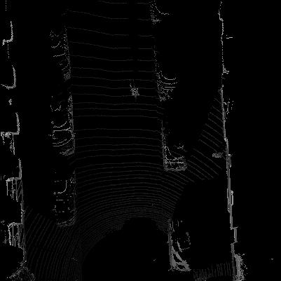
At the moment, the image is stored as a numpy array. If we wish to visualize it we could convert it to a PIL image, and view it.
# CONVERT FROM NUMPY ARRAY TO A PIL IMAGE
from PIL import Image
im2 = Image.fromarray(im)
im2.show()
We as humans are not good at telling the difference between shades of grey, so it can help to use a spectral color-mapping to make it easier for us to tell differences in value. We can do this in matplotlib.
import matplotlib.pyplot as plt
plt.imshow(im, cmap="spectral", vmin=0, vmax=255)
plt.show()
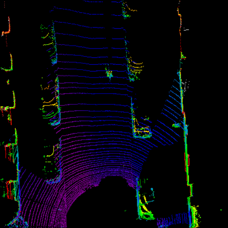
It actually encodes exactly the same amount of information as the image drawn by PIL, so a machine learning learning algorithm would for instance still be able to distinguish the differences in height, even if we humans cannot see the differences very clearly.
Complete Code
For convenience, I put together all the above code into a single function, which returns the birds eye view as a numpy array. You can then chose to either visualise it with whatever method you prefer, or plug the numpy array into a machine learning algorithm.
import numpy as np


# ==============================================================================
#                                                                   SCALE_TO_255
# ==============================================================================
def scale_to_255(a, min, max, dtype=np.uint8):
    """ Scales an array of values from specified min, max range to 0-255
        Optionally specify the data type of the output (default is uint8)
    """
    return (((a - min) / float(max - min)) * 255).astype(dtype)


# ==============================================================================
#                                                         POINT_CLOUD_2_BIRDSEYE
# ==============================================================================
def point_cloud_2_birdseye(points,
                           res=0.1,
                           side_range=(-10., 10.),  # left-most to right-most
                           fwd_range = (-10., 10.), # back-most to forward-most
                           height_range=(-2., 2.),  # bottom-most to upper-most
                           ):
    """ Creates an 2D birds eye view representation of the point cloud data.

    Args:
        points:     (numpy array)
                    N rows of points data
                    Each point should be specified by at least 3 elements x,y,z
        res:        (float)
                    Desired resolution in metres to use. Each output pixel will
                    represent an square region res x res in size.
        side_range: (tuple of two floats)
                    (-left, right) in metres
                    left and right limits of rectangle to look at.
        fwd_range:  (tuple of two floats)
                    (-behind, front) in metres
                    back and front limits of rectangle to look at.
        height_range: (tuple of two floats)
                    (min, max) heights (in metres) relative to the origin.
                    All height values will be clipped to this min and max value,
                    such that anything below min will be truncated to min, and
                    the same for values above max.
    Returns:
        2D numpy array representing an image of the birds eye view.
    """
    # EXTRACT THE POINTS FOR EACH AXIS
    x_points = points[:, 0]
    y_points = points[:, 1]
    z_points = points[:, 2]

    # FILTER - To return only indices of points within desired cube
    # Three filters for: Front-to-back, side-to-side, and height ranges
    # Note left side is positive y axis in LIDAR coordinates
    f_filt = np.logical_and((x_points > fwd_range[0]), (x_points < fwd_range[1]))
    s_filt = np.logical_and((y_points > -side_range[1]), (y_points < -side_range[0]))
    filter = np.logical_and(f_filt, s_filt)
    indices = np.argwhere(filter).flatten()

    # KEEPERS
    x_points = x_points[indices]
    y_points = y_points[indices]
    z_points = z_points[indices]

    # CONVERT TO PIXEL POSITION VALUES - Based on resolution
    x_img = (-y_points / res).astype(np.int32)  # x axis is -y in LIDAR
    y_img = (-x_points / res).astype(np.int32)  # y axis is -x in LIDAR

    # SHIFT PIXELS TO HAVE MINIMUM BE (0,0)
    # floor & ceil used to prevent anything being rounded to below 0 after shift
    x_img -= int(np.floor(side_range[0] / res))
    y_img += int(np.ceil(fwd_range[1] / res))

    # CLIP HEIGHT VALUES - to between min and max heights
    pixel_values = np.clip(a=z_points,
                           a_min=height_range[0],
                           a_max=height_range[1])

    # RESCALE THE HEIGHT VALUES - to be between the range 0-255
    pixel_values = scale_to_255(pixel_values,
                                min=height_range[0],
                                max=height_range[1])

    # INITIALIZE EMPTY ARRAY - of the dimensions we want
    x_max = 1 + int((side_range[1] - side_range[0]) / res)
    y_max = 1 + int((fwd_range[1] - fwd_range[0]) / res)
    im = np.zeros([y_max, x_max], dtype=np.uint8)

    # FILL PIXEL VALUES IN IMAGE ARRAY
    im[y_img, x_img] = pixel_values

    return im