Lidar Birds Eye Views
Summary
Today i started working on creating birds eye view images of the LIDAR data.
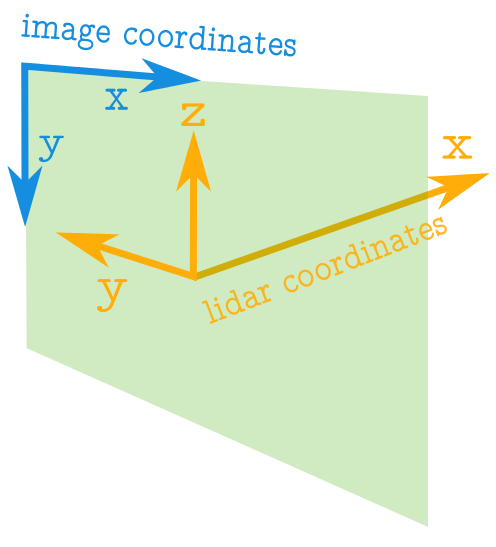
Quirks of the Lidar Coordinates
One thing to keep in mind about the LIDAR data is that the axes represent different things to what a camera photo would represent, and they point in different directions too. The following image illustrates how they differ. Notice how the x axis is actually the depth, and the horizontal axis is the y axis.
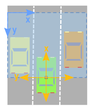
Limiting to a Rectangular Region
Instead of creating a birds eye view of every single point captured by the Lidar, it is useful to just focus in on a rectangular region of the data when looked at from the top. As for instance illustrated in the image below. Also notice how the x, and y axes will need to be swapped around, and made to point in the opposite direction when converting to image coordinates.
We will want to create a filter that only keeps points within the desired rectangle. The following code creates a 30x30m region, such that it captures 15m on either side of the car, and 30 m in front of it.
# LIMIT VIEWING RANGE - To within a desired rectangle
side_range = [-15, 15] # 10 metres on either side
fwd_range = [-0, 30]   # 30 metres in front

# INDICES FILTER - of values within the desired rectangle
# Note left side is positive y axis in LIDAR coordinates
ff = np.logical_and((x_lidar > fwd_range[0]), (x_lidar < fwd_range[1]))
ss = np.logical_and((y_lidar > -side_range[1]), (y_lidar < -side_range[0]))
indices = np.argwhere(np.logical_and(ff, ss)).flatten()

# POINTS TO USE FOR IMAGE
x_img = -y_lidar[indices]       # x axis is -y in LIDAR
y_img = x_lidar[indices]        # y axis is x in LIDAR
pixel_values = z_lidar[indices] # Height values used for pixel intensity

# Shift values so (0,0) is the minimum value
x_img -= side_range[0]
y_img -= fwd_range[0]
Simple Implementation in Matplotlib
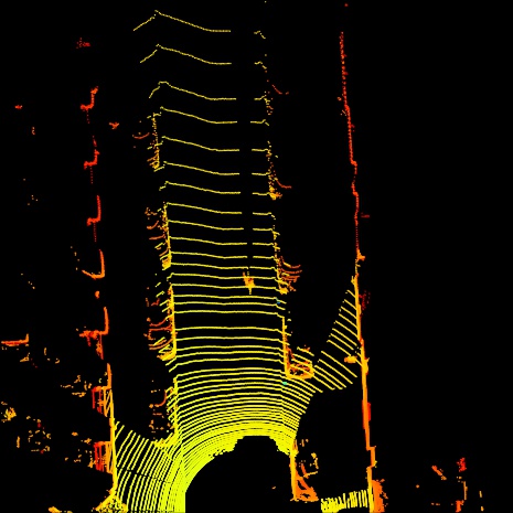
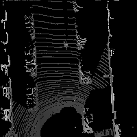
The following piece of code creates a 2D image of the points in the region by plotting them out with matplotlib, and color coding the points based on their height value.
# PLOT THE IMAGE
cmap = "jet"    # Color map to use
dpi = 100       # Image resolution
x_max = side_range[1] - side_range[0]
y_max = fwd_range[1] - fwd_range[0]
fig, ax = plt.subplots(figsize=(600/dpi, 600/dpi), dpi=dpi)
ax.scatter(x_img, y_img, s=1, c=pixel_values, linewidths=0, alpha=1, cmap=cmap)
ax.set_axis_bgcolor((0, 0, 0))  # Set regions with no points to black
ax.axis('scaled')  # {equal, scaled}
ax.xaxis.set_visible(False)  # Do not draw axis tick marks
ax.yaxis.set_visible(False)  # Do not draw axis tick marks
plt.xlim([0, x_max])  # prevent drawing empty space outside of horizontal FOV
plt.ylim([0, y_max])  # prevent drawing empty space outside of vertical FOV
fig.savefig("/tmp/simple_top.jpg", dpi=dpi, bbox_inches='tight', pad_inches=0.0)
Which creates an image like the following:
Better solution using numpy and PIL
Creating the images in Matplotlib has the advantage that we can choose pretty spectral colormappings to make it easier for us humans to distinguish ranges of values. But matplotlib is horribly slow, and will therefore be impractical if we want to create huge batches of these images as a form of data preprocessing to pass on to a machine learning algorithm.
To that extent, I created a much more efficient version of processing the images that uses numpy and PIL.
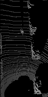
from PIL import Image
import numpy as np

# ==============================================================================
#                                                                   SCALE_TO_255
# ==============================================================================
def scale_to_255(a, min, max, dtype=np.uint8):
    """ Scales an array of values from specified min, max range to 0-255
        Optionally specify the data type of the output (default is uint8)
    """
    return (((a - min) / float(max - min)) * 255).astype(dtype)


# ==============================================================================
#                                                          BIRDS_EYE_POINT_CLOUD
# ==============================================================================
def birds_eye_point_cloud(points,
                          side_range=(-10, 10),
                          fwd_range=(-10,10),
                          res=0.1,
                          min_height = -2.73,
                          max_height = 1.27,
                          saveto=None):
    """ Creates an 2D birds eye view representation of the point cloud data.
        You can optionally save the image to specified filename.

    Args:
        points:     (numpy array)
                    N rows of points data
                    Each point should be specified by at least 3 elements x,y,z
        side_range: (tuple of two floats)
                    (-left, right) in metres
                    left and right limits of rectangle to look at.
        fwd_range:  (tuple of two floats)
                    (-behind, front) in metres
                    back and front limits of rectangle to look at.
        res:        (float) desired resolution in metres to use
                    Each output pixel will represent an square region res x res
                    in size.
        min_height:  (float)(default=-2.73)
                    Used to truncate height values to this minumum height
                    relative to the sensor (in metres).
                    The default is set to -2.73, which is 1 metre below a flat
                    road surface given the configuration in the kitti dataset.
        max_height: (float)(default=1.27)
                    Used to truncate height values to this maximum height
                    relative to the sensor (in metres).
                    The default is set to 1.27, which is 3m above a flat road
                    surface given the configuration in the kitti dataset.
        saveto:     (str or None)(default=None)
                    Filename to save the image as.
                    If None, then it just displays the image.
    """
    x_lidar = points[:, 0]
    y_lidar = points[:, 1]
    z_lidar = points[:, 2]
    # r_lidar = points[:, 3]  # Reflectance

    # INDICES FILTER - of values within the desired rectangle
    # Note left side is positive y axis in LIDAR coordinates
    ff = np.logical_and((x_lidar > fwd_range[0]), (x_lidar < fwd_range[1]))
    ss = np.logical_and((y_lidar > -side_range[1]), (y_lidar < -side_range[0]))
    indices = np.argwhere(np.logical_and(ff,ss)).flatten()

    # CONVERT TO PIXEL POSITION VALUES - Based on resolution
    x_img = (-y_lidar[indices]/res).astype(np.int32) # x axis is -y in LIDAR
    y_img = (x_lidar[indices]/res).astype(np.int32)  # y axis is -x in LIDAR
                                                     # will be inverted later

    # SHIFT PIXELS TO HAVE MINIMUM BE (0,0)
    # floor used to prevent issues with -ve vals rounding upwards
    x_img -= int(np.floor(side_range[0]/res))
    y_img -= int(np.floor(fwd_range[0]/res))

    # CLIP HEIGHT VALUES - to between min and max heights
    pixel_values = np.clip(a = z_lidar[indices],
                           a_min=min_height,
                           a_max=max_height)

    # RESCALE THE HEIGHT VALUES - to be between the range 0-255
    pixel_values  = scale_to_255(pixel_values, min=min_height, max=max_height)

    # FILL PIXEL VALUES IN IMAGE ARRAY
    x_max = int((side_range[1] - side_range[0])/res)
    y_max = int((fwd_range[1] - fwd_range[0])/res)
    im = np.zeros([y_max, x_max], dtype=np.uint8)
    im[-y_img, x_img] = pixel_values # -y because images start from top left

    # Convert from numpy array to a PIL image
    im = Image.fromarray(im)

    # SAVE THE IMAGE
    if saveto is not None:
        im.save(saveto)
    else:
        im.show()
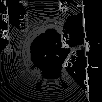
Below are some examples of this function being used. Note that although the images do not look as pretty as the ones created by Matplotlib, they still contain the same height information encoded in the pixel values. It is just more dificult for us humans to tell the difference between different shades of grey.
# View a Square that is 10m on all sides of the car
birds_eye_point_cloud(lidar, side_range=(-10, 10), fwd_range=(-10, 10), res=0.1, saveto="lidar_pil_01.png")
# View a Square that is 10m on either side of the car and 20m in front
birds_eye_point_cloud(lidar, side_range=(-10, 10), fwd_range=(0, 20), res=0.1, saveto="lidar_pil_02.png")
# View a rectangle that is 5m on either side of the car and 20m in front
birds_eye_point_cloud(lidar, side_range=(-5, 5), fwd_range=(0, 20), res=0.1, saveto="lidar_pil_03.png")
Next steps
The next step will be to follow Chen et al. 2016 and create image slices at multiple heights, and use these as aditional chanels of an image.
Also, I would like to go back to the work i left of in my previous blog post about creating "front views" of point cloud data. That was implemented using Matplotlib. I will want to create a numpy+PIL solution to make it more efficient.
Comments
Note you can comment without any login by:
- Typing your comment
- Selecting "sign up with Disqus"
- Then checking "I'd rather post as a guest"