Semantic segmentation is the task of classifying exactly which pixels belong to different classes of objects in an image. This can be particularly useful for self-driving car applications, where you would want to identify the shapes and positions of things in the environment, such as the road, other cars, cyclists, pedestrians and other obstacles.

This project makes use of the Kitti road dataset to perform the basic task of segmentation of just the road.

Several models were created, the best of which attained an Intersect over Union score of 0.885 on a validation dataset.

Data

The specific dataset used is labeled base kit with: left color images, calibration and training labels (0.5 GB), which can be downloaded with this link.

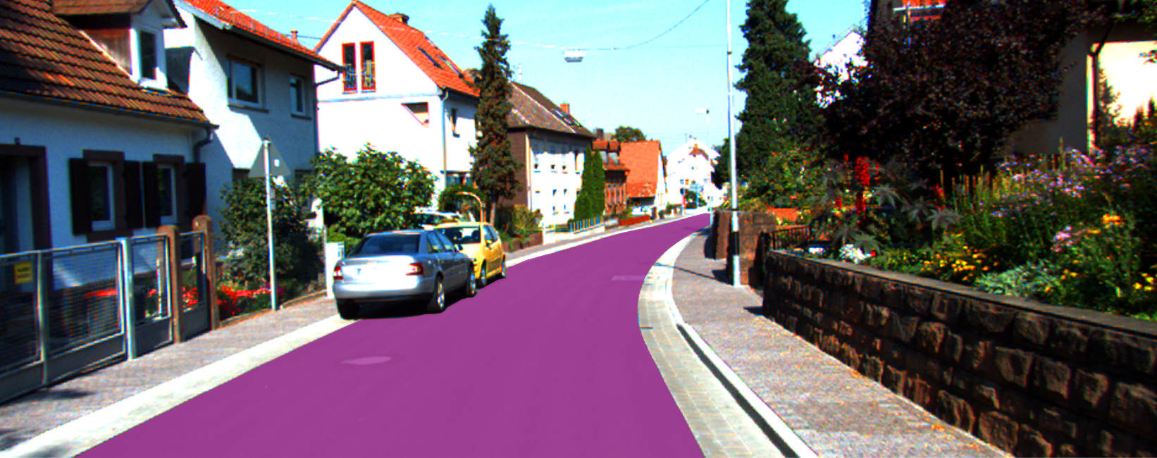
This is quite a small dataset that consists of only 289 images. Each image is 1242 by 375 pixels in size. An example of one of the images is shown below.

The input images are accompanied by two sets of label images that color code things of interest. In one set, it identifies just the lane that the car is on. In the other set, it identifies all the road. For this project, the data corresponding to all the road surface is used. These labels are RGB images that color code the road as magenta, non-road areas as red, and more road surfaces in black.

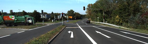
The labels images are processed to get a binary array that assigns a 1 to road surfaces, and 0 to non-road surfaces, as visualized below.

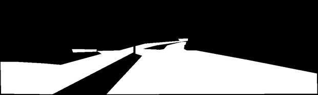
More details about how the label images were processed is outlined in this blog post

The images were resized to 299x299 pixels before feeding them into the model.

Models

Deep neural network architectures for segmentation tasks usually follow a structure similar to the one below. There are a series of convolutional operations, with the feature maps becoming downsampled along the spatial dimensions. These are then followed by upsampling layers that combine some information from previous layers.

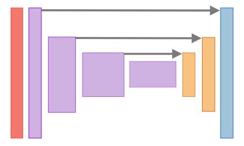
For this project, an inception V3 architecture was used for the downsampling portion of the segmentation. This was then followed by transpose convolutions for the upsampling portion. The outputs of all the inception v3 layers just before a downsampling operation was performed were passed along as skip connections. These skip connections had a 1x1 convolution applied to them. The output of that was combined with the output of the deconvolutional layer through elementwise addition.

Pretrained weights for the inception V3 portion of the architecture were used. These were trained on the imagenet dataset and provided by the Tensorflow project. The link to the file that was used is here. The remaining variables were initialized randomly using Xavier initialization.

Several different models were trained, with slight variations on the architecture. The two best ones are outlined below.

C02

• Dropout was applied to the output of the inception layers that connected to the before skip connections
• Skip connections perform a 1x1 convolution and then batchnorm but no activation function.
• Uses batchnorm in the upsampling layers.
• No activation function was applied to the upsampling layers.

D01

• Dropout was applied to the output of the inception layers that connected to the before skip connections
• Skip connections perform a 1x1 convolution but no batchnorm or activation function.
• No batchnorm in the upsampling layers.
• No activation function was applied to the upsampling layers.

Training

Given that the dataset was so small, only 33 of the images were set aside for validation, leaving 256 for training. This was accompanied by data augmentation steps that would randomly perform the following operations on each batch of images.

• synthetic shadows
• rotation
• randomly sized crops
• left-right flip
• brightness
• contrast
• blur
• noise

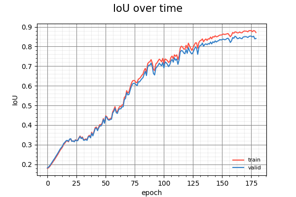
Below is the training curves for model C02. It depicts the progress of the Intersect over Union score against each epoch of training. It is accompanied by an animation of how it visually performs on validation images that it did not see during training. The timesteps for the frames in the animation is once every 10 epochs. The blue overlayed label is the ground truth. Red represents the prediction, and magenta represents where the prediction overlaps with the ground truth.

And below is the training curves and visualization for the D01 model.

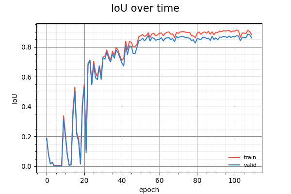
It is interesting to note how the two models make progress. The C02 model starts by predicting everything as a road and whittles the non-road regions away, like a sculptor. The D01 model, on the other hand, builds up from a tiny region.

Limitations

The number of training images is quite small, and don't contain many variations in the types of roads and lighting conditions. Even with random data augmentation steps, it is difficult for the trained models to adapt to different kinds of roads. For instance, when applied to a windy road with lots of variations in lighting, the models do quite poorly.

Sample video of model C02 on a windy road with big changes in lighting conditions.

Sample video of model D01 on a windy road with big changes in lighting conditions.

Model D01 is quite resilient to changes in lighting, and dark shadows, however, it only detects the current lane the car is in. Model C02 on the other hand captures more of the road, but it doesn't adapt well to differences in lighting conditions and does very poorly when parts of the road contain shadows.

Links

The source code for this project is located on Github.

Credits

• The base video used in the windy road demonstration is courtesy of Udacity.
• The road scene image used for the banner image is taken from the Kitti Road Dataset.