Inputs, Labels, and Outputs

Inputs

The input data used for segmentation are just regular images. They could be RGB images or just greyscale images. There is nothing different about input data you would use for a semantic segmentation task compared to an ordinary image classification task.

Labels

The labels data for training can come in one of several different forms, depending on the dataset you download.

The idea is that we would like to have class labels for each pixel of the input image. As such, the data usually gets packaged as images (or arrays representing a batch of images).

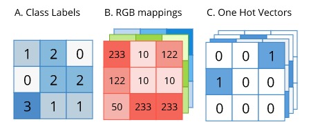
Sometimes it gets packaged as greyscale images, where the pixel intensity represents the class id (as in format A in the diagram above). This method can be the easiest to work with. It allows for a small file size for distribution and is easy to make use of directly in most deep-learning frameworks without having to do any processing.

But sometimes the data is stored as RGB images, where different classes of object will have some arbitrary RGB color representing it (as in format B in the diagram above). This method is most convenient for visualizing the labels data since you can view them using any library or program that opens regular images. It requires no extra processing steps to visualize what the segmentation labels look like. However, it does involve some pre-processing before it can be used in a deep learning pipeline. The RGB values need to be mapped to either class labels, or One Hot Vector representations. It also uses up more memory than format A.

The format that is most readily compatible with any deep learning framework is format C, where each pixel is encoded as a one-hot vector, with a value of 1 for the class it represents. Even if the deep learning framework you use accepts the labels data as class ids, as in format A, it will convert that data to one-hot encoding behind the scenes.

Outputs of the Segmentation Model

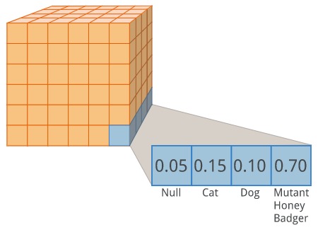
The output of a semantic segmentation architecture is a tensor of shape [n_samples, height, width, n_classes]. It has the same width and height as the original input images. The final axis contains the predicted probability distributions of the different classes, for a particular pixel (after we feed it through a softmax). We can think of each pixel as making a guess "I am most confident that this pixel belongs to a mutant honey badger". The image below shows what the output data would look like for a single sample.