Creating Height Slices of Lidar Data
Summary
Today I worked on extending the work I did yesterday for creating birds-eye view images of the Lidar data from the Kitti dataset. The task was to slice the data into height slices, and use each of those slices as separate channels of an image.
Heights as Channels
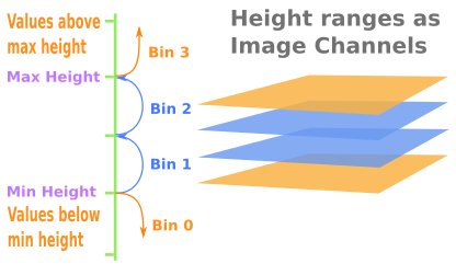
Usually when we think of numerous channels in an image we think of color channels, eg RGB. But Chen et al 2016 did something quite interesting. They used multiple channels as a way of encoding height data. In yesterdays blog, I encoded the height as pixel intensities (values between 0-255).
The idea is to create slices at different heights, and use those slices as channels of the image. We can accomplish this in numpy by binning the height values, and using the bin indices as channel indices when creating the image arrays. The following diagram illustrates the general idea.
And below is code to achieve this.
# ASSIGN EACH POINT TO A HEIGHT SLICE
n_slices = 8
# n_slices-1 is used because values above max_height get assigned to an
# extra index when we call np.digitize().
bins = np.linspace(min_height, max_height, num=n_slices-1)
slice_indices = np.digitize(z_points, bins=bins, right=False)
An advantage of encoding the height data as separate chanels of the image is that we can therefore pack aditional information in the pixel intensities, such as reflectance values.
Assigning the points to their corresponding position in the image is now just a matter of doing something like the following.
im = np.zeros([y_max, x_max, n_slices], dtype=np.uint8)
im[y_pos, x_pos, slice_indices] = reflectance_vals
Slices Function
The function created in yesterdays blog can now be updated with the above snippets of code, so we get something like this:
import numpy as np

# ==============================================================================
#                                                                   SCALE_TO_255
# ==============================================================================
def scale_to_255(a, min, max, dtype=np.uint8):
    """ Scales an array of values from specified min, max range to 0-255
        Optionally specify the data type of the output (default is uint8)
    """
    return (((a - min) / float(max - min)) * 255).astype(dtype)


# ==============================================================================
#                                                        BIRDS_EYE_HEIGHT_SLICES
# ==============================================================================
def birds_eye_height_slices(points,
                            n_slices=8,
                            height_range=(-2.73, 1.27),
                            side_range=(-10, 10),
                            fwd_range=(-10, 10),
                            res=0.1,
                            ):
    """ Creates an array that is a birds eye view representation of the
        reflectance values in the point cloud data, separated into different
        height slices.

    Args:
        points:     (numpy array)
                    Nx4 array of the points cloud data.
                    N rows of points. Each point represented as 4 values,
                    x,y,z, reflectance
        n_slices :  (int)
                    Number of height slices to use.
        height_range: (tuple of two floats)
                    (min, max) heights (in metres) relative to the sensor.
                    The slices calculated will be within this range, plus
                    two additional slices for clipping all values below the
                    min, and all values above the max.
                    Default is set to (-2.73, 1.27), which corresponds to a
                    range of -1m to 3m above a flat road surface given the
                    configuration of the sensor in the Kitti dataset.
        side_range: (tuple of two floats)
                    (-left, right) in metres
                    Left and right limits of rectangle to look at.
                    Defaults to 10m on either side of the car.
        fwd_range:  (tuple of two floats)
                    (-behind, front) in metres
                    back and front limits of rectangle to look at.
                    Defaults to 10m behind and 10m in front.
        res:        (float) desired resolution in metres to use
                    Each output pixel will represent an square region res x res
                    in size along the front and side plane.
    """
    x_points = points[:, 0]
    y_points = points[:, 1]
    z_points = points[:, 2]
    r_points = points[:, 3]  # Reflectance

    # FILTER INDICES - of only the points within the desired rectangle
    # Note left side is positive y axis in LIDAR coordinates
    ff = np.logical_and((x_points > fwd_range[0]), (x_points < fwd_range[1]))
    ss = np.logical_and((y_points > -side_range[1]), (y_points < -side_range[0]))
    indices = np.argwhere(np.logical_and(ff, ss)).flatten()

    # KEEPERS - The actual points that are within the desired  rectangle
    y_points = y_points[indices]
    x_points = x_points[indices]
    z_points = z_points[indices]
    r_points = r_points[indices]

    # CONVERT TO PIXEL POSITION VALUES - Based on resolution
    x_img = (-y_points / res).astype(np.int32) # x axis is -y in LIDAR
    y_img = (x_points / res).astype(np.int32)  # y axis is -x in LIDAR
                                               # direction to be inverted later
    # SHIFT PIXELS TO HAVE MINIMUM BE (0,0)
    # floor used to prevent issues with -ve vals rounding upwards
    x_img -= int(np.floor(side_range[0] / res))
    y_img -= int(np.floor(fwd_range[0] / res))

    # ASSIGN EACH POINT TO A HEIGHT SLICE
    # n_slices-1 is used because values above max_height get assigned to an
    # extra index when we call np.digitize().
    bins = np.linspace(height_range[0], height_range[1], num=n_slices-1)
    slice_indices = np.digitize(z_points, bins=bins, right=False)

    # RESCALE THE REFLECTANCE VALUES - to be between the range 0-255
    pixel_values = scale_to_255(r_points, min=0.0, max=1.0)

    # FILL PIXEL VALUES IN IMAGE ARRAY
    # -y is used because images start from top left
    x_max = int((side_range[1] - side_range[0]) / res)
    y_max = int((fwd_range[1] - fwd_range[0]) / res)
    im = np.zeros([y_max, x_max, n_slices], dtype=np.uint8)
    im[-y_img, x_img, slice_indices] = pixel_values

    return im
And here is an example of this function being used on a frame of the Kitti dataset's lidar data. Given that the Lidar sensor is positioned 1t 1.73m from the ground, the following will capture slices that are clipped between 27cm below a perfectly flat road surface, and 2m above such a flat road surface. It creates 8 height slices. It looks at a region 10m on either side of the car, and 20m in front, at a resolution of 10cm.
im = birds_eye_height_slices(lidar,
                        n_slices=8,
                        height_range=(-2.0, 0.27),
                        side_range=(-10, 10),
                        fwd_range=(0, 20),
                        res=0.1)
Calling this function returns a 200x200x8 nunmpy array. It is not actually possible to save (or view) this as an actual image, eg a PNG, because image libraries are only really built to interpret a maximum of about 3 or 4 channels in a small number of common ways, eg for coding red,green, blue and alpha. But a convolutional neural network will not mind at all, you can create one to take in as many channels as you like.
Visualising
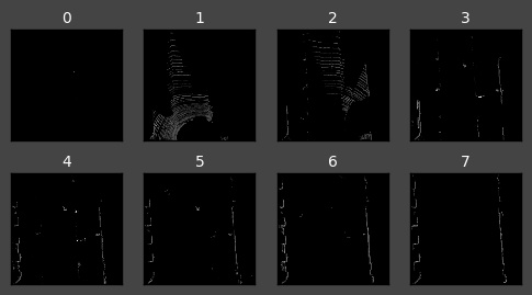
In order to prove to ourselves that what has been created is correct, we can visualise the array one layer at a time.
# VISUALISE THE SEPARATE LAYERS IN MATPLOTLIB
import matplotlib.pyplot as plt
dpi = 100       # Image resolution
fig, axes = plt.subplots(2, 4, figsize=(600/dpi, 300/dpi), dpi=dpi)
axes = axes.flatten()
for i,ax in enumerate(axes):
    ax.imshow(im[:,:,i], cmap="gray", vmin=0, vmax=255)
    ax.set_axis_bgcolor((0, 0, 0))  # Set regions with no points to black
    ax.xaxis.set_visible(False)     # Do not draw axis tick marks
    ax.yaxis.set_visible(False)     # Do not draw axis tick marks
    ax.set_title(i, fontdict={"size": 10, "color":"#FFFFFF"})
fig.subplots_adjust(wspace=0.20, hspace=0.20)
fig.show()
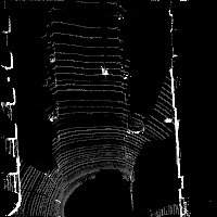
We can also visualise that there has been no loss of information by collapsing all the layers together into a flat image. The following code summarises the elements along the channels by summing them up and clipping them to within the range 0-255.
from PIL import Image
b = np.clip(np.sum(im, axis=2), a_min=0, a_max=255).astype(np.uint8)
Image.fromarray(b).show()
Next Steps
The next step will be to go back to the code created in this blogpost from a few days ago to create the "front view" images more efficiently without using matplotlib.
After that, it is a matter of processing some samples and attempting to create a neural network that can use those inputs to detect vehicles in the scene and their position and orientation.
Comments
Note you can comment without any login by:
- Typing your comment
- Selecting "sign up with Disqus"
- Then checking "I'd rather post as a guest"